Making maps in New York - the street map

To put together any sort of map that tells a story, you need two kinds of mapping data. The first is a basemap: a general picture of the land, and the second is the thematic data: the stuff you add to the basemap to tell your story. I'm not quite ready to tell the story of Niskayuna's nature preserves yet, but at least I know where they are, and I've found sources for basemap data. Let's have a look at some workflows for putting the basemap together.

Andy Arthur, in his tutorial on QGIS, gives one approach, which starts from the 7.5-minute quadrangle maps published by the New York State Department of Transportation. While these maps are aligned to the same grid as the better-known USGS topographic maps, they are not the same maps; they are somewhat more up to date than the USGS series, and unlike the scanned USGS maps, they are available in four individual layers, one per ink color. They're available from the New York State GIS Clearinghouse - one of the two major GIS repositories for New York. (The other is the Cornell University Geospatial Information Repository [CUGIR].)

The maps in question consist of one sheet for each of the nearly one thousand quadrangles that make up New York. Each sheet has four separate GeoTIFF files, one per ink color. On the traditional New York State topos that I used when I worked for a county government in the 1970s, the printing layers were:

• Plan (black) - Overprinted features in black. These are a mix of everything: cultural features (roads and buildings), political features (boundaries and jurisdiction names), place names, and even some hydrology (linear features like streams, and patterned features like marshes).


• Hydrology (blue) - Polygons giving surface water cover - rivers and lakes.


• Topography (brown) - Contour lines giving elevations.


• Built-up areas (yellow on NYS maps, pink on USGS ones) - A shaded overprint marking the area where habitation is so dense that individual buildings are not shown in the plan.

Andy Arthur's tutorial on QGIS gives quite a comprehensive description for dealing with these layers in QGIS, so I won't repeat it here.

Combining these four layers for the Niskayuna quadrangle gives a reasonably attractive map:

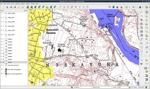
It's certainly a technique that I'll keep in my back pocket. But it's not the way that I've decided to go, for several reasons:

• The maps are raster graphics, which means that they won't scale gracefully. They will pick up pixel artifacts when printed at any other scale than 1:24000, 508 pixels to the inch. (Why 508? Not sure!)


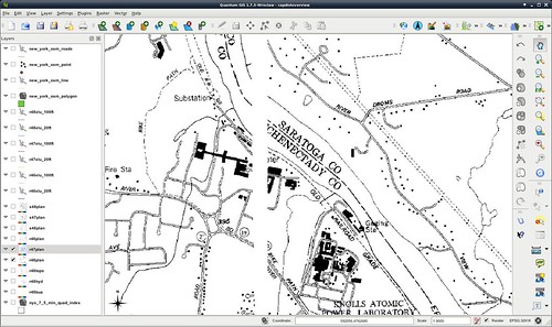
• The maps are old data: the one that I show in the screenshot was produced in 1980. A lot has changed in 32 years.


• The maps as scanned are missing stuff along the margins of the region. If I take two quads and lay them together, they don't quite join. It appears that the scans have been cropped a bit too aggressively.

The USGS digital raster graphics do not have the problem of failing to join up, but they are, for the most part, even older. (Also, they have the problem that they are in color and can't be separated readily.) The newer USTOPO maps are not really intended for GIS use (and don't play all that well with GIS software): it's better to go back to the GIS sources that make them up, which are for the most part publicly available.

The first thing that maps usually need to show is context: "where is this map relative to the street where I live?" is the first question to answer. So most maps that I produce will need a road map. Most road maps in the US eventually draw on the TIGER maps maintained by the Census Bureau. One public source that draws heavily on TIGER, but then crowdsources additional data, is the OpenStreetMap project. It's become quite good; if all you need is a street map, it's probably serviceable as a basemap. In any case, it should serve well as a starting point for an overlay of cultural features.

The data in GIS form for just the state of New York are available from http://downloads.cloudmade.com/americas/northern_america/united_states/new_york. They are encoded in an OpenStreetMap-specific format, but QGIS (at least with plugins) can deal with it.

But there's an issue: The OSM data set is big. The New York data alone are about three gigabytes after decompression. QGIS becomes unacceptably slow and unstable when trying to work with data of this size. Here, PostGIS (which I mentioned in the last post) comes to the rescue. It allows the map data to be saved in a PostgreSQL database, and allows QGIS to load only the data it needs to render a particular map.

So, after installing all the tools that PostGIS needs, we follow the instructions to create a spatially enabled database. Next, we use the osm2pgsql utility to load up the OpenStreetMap data into the database from the command line:

osm2pgsql -S /usr/share/osm2pgsql/default.style -E 32618 -d gis -k -s -p new_york_osm new_york.osm

Go to lunch. it takes a while.

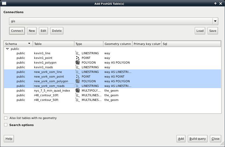
OK, once it's done, "Add PostGIS Layer" will allow selection from the database and adding the layer to QGIS. It brings up a dialog that looks as shown below, and I select all the layers that I just put in using 'osm2pgsql', and add them.


After it chugs for a little while, it shows me the graphics.


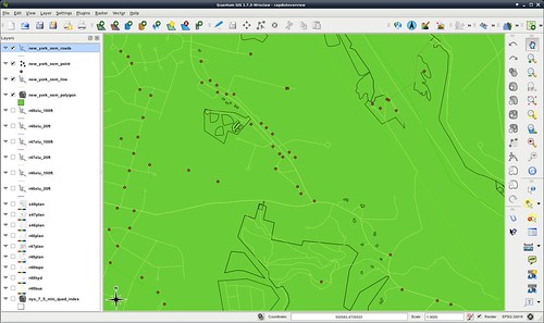
Yes, they look like hell. We'll get around to that. The point is that the streets and boundaries are there. But right now, we need more data. The map I want is more than a road map.
The next post will discuss topography.