Making maps in New York - topography

When we left off, we had a map project that had OpenStreetMap data in a PostGIS database, If the symbols were properly styled, having this data set alone could produce rather a pretty map. But it's far from ideal as a walking map - for one thing, I want to know when I'm walking whether I should expect to be going up and down steep hills. Of course, the customary way for a map to present this information about topography is to mark up the map with a series of contour lines - lines joining points at the same elevation.

We saw before that we could get contours from the 'topo' layer of the NYS DOT quadrangles, but we also saw that doing so had problems, because (1) the quads appear to be trimmed off at the margins, and (2) the resulting images scale poorly because they are raster images. So let's attempt a different data source.

The US Geological Survey publishes a Digital Elevation Model (DEM) of the United States, meshing it into a fine grid (the point spacing is 1/3 of a second of arc) with the elevation reported at each point. The CUGIR server makes the data available by quadrangle. So we begin by downloading the model for the quadrangles of interest, and unpacking the resulting files. (They wind up placing a ZIP within a ZIP, so have to be unpacked twice.) The result is that we have a bunch of files with the extension '.dem' that have the required data.

If the Python-GDAL tools are installed, then QGIS can take these data and produce contour lines in vector format. These lines will scale gracefully with changes in map scale. The way to get them is to open up a fresh QGIS project (or it's all right temporarily to add layers to an existing one), and load in a DEM file as a raster layer. When it's loaded, right-click on it in the 'Layers' display and choose 'Set Project CRS from Layer' (if you're working in an existing project, it will have to be set back afterward.) This will change the co-ordinate reference of the project to EPSG:26718 (NAD27 Universal Transverse Mercator Zone 18N), which we need because the DEM files use the old 1927 North American Datum coordinate system.

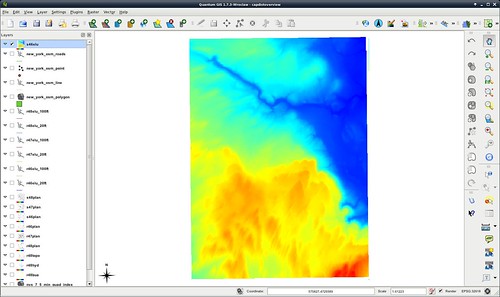
Once you've loaded the layer and adjusted the coordinate frame, choose 'Zoom to Layer' from the view menu. You'll see a gray rectangle that shows the part of the ground that the model covers.
You can color this area according to elevation, if you like, by right-clicking on the layer, choosing 'Properties' from the menu, selecting the 'Style' tab and changing the 'Color Map' to
'Pseudocolor'.


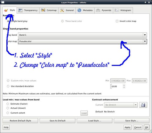
Now you'll see the same area in false color: reds are high elevations, and blues are low.


Since I'm an American, I tend to prefer maps with contours in feet rather than the more sensible metres. The DEM files have metric elevation, so to produce foot contours, we need to rescale them. Choose 'Raster Calculator' from the 'Raster' menu, and carry out the steps in the picture:

Enter the name of a GeoTIFF file to be created that will contain the elevation data in feet

Click 'Current Layer Extent' to make the new file have the same dimensions as the old

Set the output format to 'GeoTIFF' and select 'Add result to project' so that you can preview the conversion

Use the left-hand list to choose the layer to convert, and complete the expression (layer / 12.0 / 0.0254), which converts feet to metres

Click 'OK'

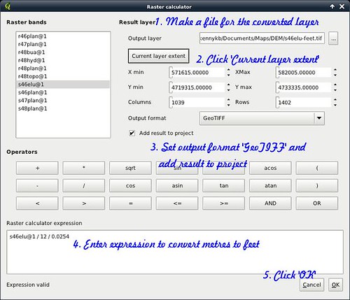
You'll get another gray rectangle that you can convert to pseudocolor to determine that the metres-to-feet conversion was successful.

Now you're ready to produce the actual contour lines. Carry out this task by pulling 'Raster->Extract->Contour' from the menu bar. You'll get a dialog box:

Select the feet-based raster that you just created as the input file

Choose the location of a new 'shp' file (together with the other files that go with it) as the output file. The file must not exist, but the containing directory must exist.

Enter an appropriate contour interval. For the rolling hills of upstate New York, at scales 1:24000 and finer, 20 feet is pretty good.

Check 'Load into canvas when finished' to be able to review the work

Click 'OK.' Don't close the window yet.

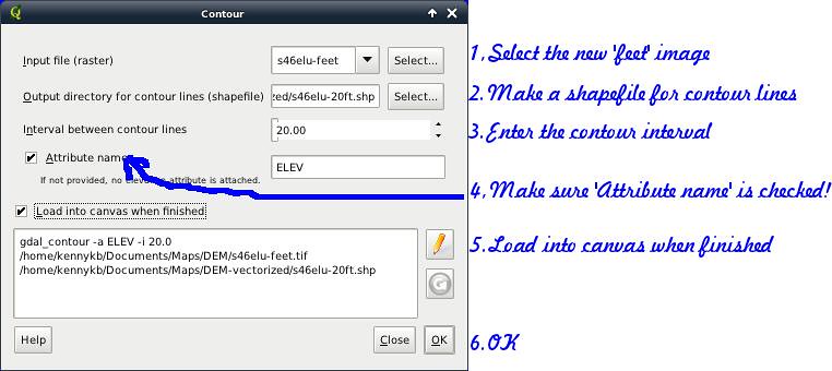
You should now see contour lines overlaid on top of the color image - uncheck both image layers in the list to make them more visible. If they look good, then we will also want index contours - highlighting of every fifth contour line to make them easier to read. Go back to the contour dialog, change both '20's to '100's, and click 'OK' again. You'll get a second set of contours overlaying the first.

These steps have to be done for every DEM quadrangle that you download. Given the title of this blog, and my penchant for scripting languages, I really ought to script this workflow. But I haven't done it yet (partly because I'm not positive that I have it completely right).

Once you have all the contours, it's advantageous to put them in the database. (If you have a large number of contours that don't appear in a particular view, QGIS can use database queries to filter them, and render much faster.) For this, we go back to the command line, and do:

For the first file:

$ /usr/lib/postgresql/9.1/bin/shp2pgsql -c r46elu_100ft.shp kbk_100ft_contours \
     | psql -d gis > /dev/null

(The -c asks to create a database table afresh, and the remaining arguments are the first .shp file and the name of the table.)

For each subsequent file except the last:

$ /usr/lib/postgresql/9.1/bin/shp2pgsql -a r46elu_100ft.shp kbk_100ft_contours \
     | psql -d gis > /dev/null

(The -a asks to append to an existing table in the database.)

And for the last file:

$ /usr/lib/postgresql/9.1/bin/shp2pgsql -a -I r46elu_100ft.shp kbk_100ft_contours \
     | psql -d gis > /dev/null

(The -I option asks to create a spatial index over the layer after loading it.)

These steps must be carried out for both 20- and 100-foot contours. Once again, I ought to script it. But I haven't done that yet.

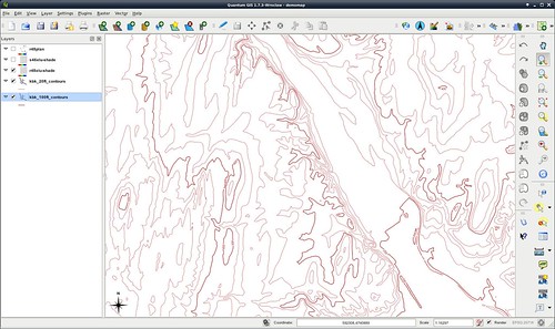
So now, start with a clean slate again in QGIS, and do 'Layer->Add PostGIS layer', selecting the two layers we just built. Remember to use EPSG:26718 as the layer coordinate reference system! These contour lines will be the ones we'll have on the finished map, so we might as well style them prettily. Bring up the 'Properties' on the 20 foot contours, change the color to brown and the line width to 0.18 mm (1/2 point). Then bring up the 'Properties' on the 100 foot contours, and change the color to brown and the line width to 0.35 mm (1 point). Finally, select the 100 foot contour layer, and pull 'Layer->Labeling'. Settings that I find attractive are:

• Check 'Label this Layer' and select the 'elev' field


• Choose the font 'Liberation Sans' 8-point italic, in the same shade of brown as the contours.


• Use a 1-mm buffer


• In the 'Advanced' tab: Placement parallel, on the line, at a distance of zero, oriented to the line. Medium priority. Suppress labeling for features smaller than 10 mm. Features don't act as obstacles.


• In the 'Engine Settings' dialog, 'Popmusic Tabu' seems to give a trifle better placement for the contour labels than the default 'Chain'.

So now we have a serviceable set of contour lines.


Don't throw out the original raster images, we may be reusing them to do hill shading later.
In the meantime, we'll move onward to hydrography in the next installment.